Introduction
Deep learning architectures have greatly impacted the success of machine learning in modern applications. However, these applications require training large quantities of data to ensure functionality, a process which can be elaborate and require significant time expenditure. Thus, active learning frameworks were introduced in order to improve data efficiency in deep learning.
Active learning targets real-world situations in which labeled data are scarce, unlabeled data are abundant, and labeling a large quantity of data is difficult, costly, and time-consuming. Therefore, a proper labeling scheme that would reduce the number of labels required to train a classifier was proposed.
Data
The dataset used was the MNIST dataset for handwritten digits.
http://yann.lecun.com/exdb/mnist/
The MNIST dataset contains 55,000 labeled images in the training set and 10,000 images in the test set. I assumed that only a limited proportion of images was labeled in order to implement active learning techniques.
Predictive Model
The model used to build an image classifier was the Convolutional Neural Network (CNN) using the machine learning library TensorFlow.
First, I trained the CNN model on the entire MNIST dataset to ensure that it could generalize from the training data to unseen data by measuring the performance of the learned model on the test set that is separate from the training set.
Second, I assumed only 50 images were labeled from the training set and implemented active learning techniques.
Finally, I determined the best technique based on the accuracy of the test set and the behavior of the learning curve.
Active Learning
In this project, the focus was on a pool-based active learning process. Pool-based active learning consists of two main engines: a learning engine and a sampling engine.
The model was initially introduced and trained on a small set of labelled data to build a predictive model. Then, based on evaluating the informativeness and the value of instances, the learning algorithm would determine which instances to label from the unlabeled pool. Since there was in fact no exact measure of the value, I estimated the value by implementing uncertainty measures that assume that instances with higher classification uncertainty are most critical to the label. Those instances were then added into the labelled set, and the learning engine constructed a new classifier based on the updated set. The model’s performance improved as the number of labelled data increased after each iteration. This process was run repeatedly, and the active learner iteratively selected informative query instances until I depleted the budget.
This technique was computationally intensive and required evaluating the entire data set after each iteration. Despite some shortcomings, however, this process has a wide range of applications from text and image classification to speech recognition and cancer diagnosis.
Query Selection Strategies
Random Sampling
When using the random sampling method, the active learner chooses instances at random to query their actual labels. It then adds the chosen instances into the labelled set to retrain the classifier.
This method does not choose instances that are representative of the underlying distribution. However, as seen in the Figure 1, the learning curve increments substantially until it reaches a 94% accuracy score on the test set.
Figure 1: Learning Curve of Random Sampling
Most Confident
In this method, I queried instances about which the active learner was most certain. Although I had already determined that the decision for query selection would be based on uncertainty measures, I was unsure how the model would perform when choosing instances with high probability predictions.
My findings indicated that random sampling performed better than the most confident method throughout the entire learning curve, as seen in Figure 2. Thus, I concluded that the most confident approach was less favorable due to its querying of irrelevant or redundant instances that add no value to the existing labelled set.
Figure 2: Learning Curve of Random Sampling and Most Confident
Uncertainty Sampling
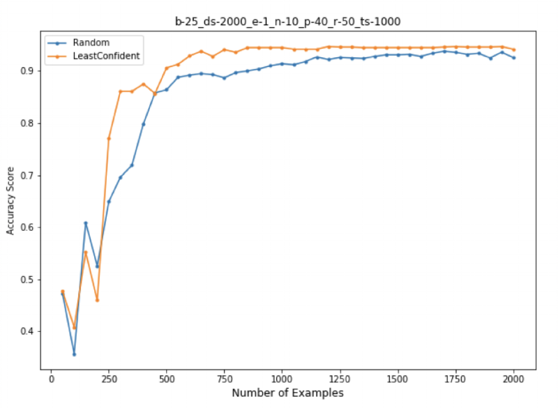
Uncertainty sampling involves the active learner querying instances for which it has the least confidence in the most likely label. Here the focus would be on instances closest to the decision boundary, assuming it can adequately explain them in other parts of the input space of the unlabeled instances. As a result, it avoids requesting labels for redundant or irrelevant instances and thus is more accurate than random sampling.
There are several techniques with which to measure uncertainty. I selected the label probability technique, which can be approached using either the least confident method or the maximum entropy method.
The least confident method queries instances whose predictions are the least confident. This method considers information about only the most probable label and discards information about the remaining label distribution.
Figure 3: Learning Curve of Random Sampling and Least Confident
Alternatively, the maximum entropy method queries instances whose label entropies are at the maximum. The probability values of the unimportant classes largely determine the measured entropy value. In other words, when computing entropies, the small probability values of unimportant classes will have a greater contribution to the entropy score, resulting in a higher entropy value even though the classifier is more confident about the classification example.
Entropy is a measure of uncertainty. If an unlabeled instance in the pooled set has a distribution with a higher entropy, this would indicate that the classifier is more uncertain about its class membership
Figure 4: Learning Curve of Random and Uncertainty Sampling
Uncertainty sampling outperformed random sampling and reached the non-change state in accuracy, with fewer labeled instances having only 800 examples and a 97% accuracy score.
Graph-Based Approach using Pairwise distance
In the graph-based method, instances are represented by vertices in a graph with edges encoding the distance between nodes. Distance serves as a notion of similarity (or dissimilarity) between instances. I captured this notion of similarity using pairwise distances. Distances are first computed for the predictions on the entire dataset then queried to label the instance that is furthest from the other labeled instances. The labeled set is then updated with the new instance, and the next furthest instance from the updated labeled set is chosen. This process is repeated until the size selection needed is reached. I then update the classifier with the new labeled data to leverage its knowledge in choosing which instances to query next.
This method handles high-dimensional data, and therefore it outperformed other active learners throughout the entire learning curve. In addition, label uncertainty on instances can be reduced because the label of the unlabeled instances is predicted by nearby labelled instances.
Figure 5: All Active Learners Curves
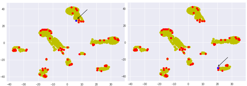
The T-SNE library was used to visualize the images. Unlabeled instances, which in this project includes 1550 examples, are shown in green. Labeled instances with only 50 labelled examples are shown in red, and instances where the active learner will query its actual label are shown in blue.
Figure 6 shows the very first iteration after querying 50 instances one at a time. It is noteworthy that the location of choosing instances moves further away from the labeled instances after each update of the labelled set. The arrow depicts the location of the chosen instance.
Figure 6: Visualization of instances for the first and second instance
Figure 7: Visualization of instances for the third and forth instance
Figure 8: Visualization of instances for the twenty-fourth and twenty-fifth instance
Exploratory Data Analysis
Stopping Criteria
Obtaining a high accuracy score on the test set would not warrant a stop in labeling. The active learner can be stopped, however, to query for more labels if the performance eventually fails to improve significantly—in other words, after a certain threshold where the accuracy reaches a non-change state.
One such occurrence of this is shown in Figure 9. Since the accuracy reached a non-change state with approximately 800 examples, the requests for more labels were discontinued. In Figure 10, the first 500 examples were examined more closely in order to demonstrate the stopping criteria with a different data size. Significantly, none of the active learners reached the steady state, and random sampling performed better than maximum entropy. This is clearly noted when comparing the graph in Figure 10 with that in Figure 9, the latter of which includes 2000 examples in the labeled set.
Figure 9: Learning Curves with Threshold at 800
Figure 10: Learning Curves with 500 Labelled Examples
Data Efficiency
I examined the significance of querying fewer data points and demonstrated how the model would perform with fewer instances.
In Figure 11, the total data size from which the active learner will choose is 20000 examples instead of 2000 examples. As shown in the figure, there are four learning curves with 5,10, 50, and 100 queries per step. The curve with 5 queries had the highest accuracy score after the threshold point. This reinforces the concept of informativeness of the examples being selected with few data points.
Figure 11: Learning Curves with Different Steps per Rating
Computation time is proportional to the number of queries selected. In table 1, the running time is inversely proportional to number of steps per rating. Therefore, it is important to choose the optimal number of queries to maximize efficiency while maintaining a favorable balance between computational time and accuracy score.
Table 1. Computational Time for Different Steps Per Rating
Supervised Learning
Supervised learning in deep learning frameworks must be trained on a large amount of labeled data. The results shown in Figure 12 are based on 2000 labelled examples. The learning curve depicts the outcome of 2000 examples chosen randomly from the labeled set and demonstrates fluctuations, which confirms that more labeled data should be fed into the model to build a robust classifier.
Additionally, if I am to assume that only 50 examples are labeled and that I trained the model using those examples, as I did in the active learning process described above, I will achieve an accuracy score of approximately 45%. So, if we allow the learning algorithm to choose the data from which to learn, it can outperform supervised learning.
Figure 12: Supervised learning Curve
Conclusion
I can conclude that data efficiency can be achieved in deep learning through active learning, and active learning can overcome the labeling bottleneck by reducing the number of labeled data required to train a classifier. In this project, the method that worked best when dealing with high dimensional data was the graph-based approach. This method achieved higher accuracy levels than other strategies by sampling more informative instances than other active learning methods.
Active learning can be implemented to address real-world problems where labeling instances is costly and time-consuming. Currently, budget restrictions and economic factors are the main stopping criteria for labeling, and different examples have different labeling costs. However, as further research is conducted with regards to the potential applications of active learning, an increase in the use such methods may be seen.


